Time and Space Complexity in Practice

Big O is a language for describing how resource use grows as input size grows. It is not a stopwatch, a ranking of every implementation, or a promise about latency on a particular machine. This guide builds on the Big O introduction with a repeatable way to analyze code and choose an implementation.

Read the input constraints first

#

Before selecting an algorithm, find the maximum input size, whether input is sorted, whether duplicates are allowed, and whether the program has a time or memory limit. An O(n²) approach can be ideal for a list of 20 items; an O(n log n) approach may be necessary for millions. Constraints tell you which growth rates are plausible.

Count the work in layers

#

Consider checking whether a list contains a duplicate. A direct nested scan compares pairs and can take quadratic time:

def has_duplicate_slow(values):
    for i in range(len(values)):
        for j in range(i + 1, len(values)):
            if values[i] == values[j]:
                return True
    return False

The inner loop runs fewer times as i grows, but the total comparisons are still n(n - 1) / 2, which is O(n²). A set trades extra memory for expected constant-time membership checks:

def has_duplicate(values):
    seen = set()
    for value in values:
        if value in seen:
            return True
        seen.add(value)
    return False

This version takes expected O(n) time and O(n) additional space. “Expected” matters: hash tables provide expected performance under ordinary hash distributions, while collisions can affect worst-case behavior.

Time and space are separate budgets

#

An optimization often moves work from one resource to another. A set prevents repeated scans but stores data. Merge sort uses O(n) auxiliary space for predictable O(n log n) time. An in-place algorithm can reduce extra memory while doing more work or becoming harder to reason about.

The right choice depends on the budget: a memory-constrained device, a latency-sensitive request, and a one-off offline script can reasonably use different algorithms.

Compare growth, then measure real code

#

The curves below are normalized to 1 at n = 1, so they show shape rather than measured time. Exponential growth quickly leaves the useful range; the exact crossover between practical implementations depends on constants, hardware, language, and input distribution.

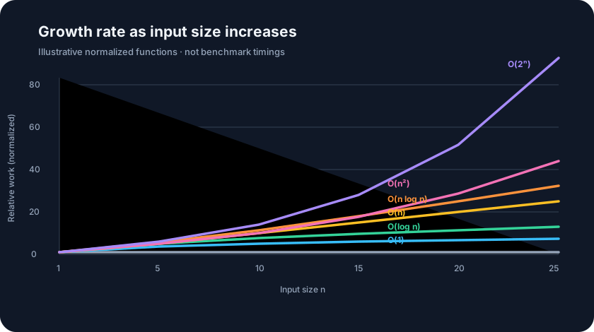
Big O intentionally ignores constant factors. For small inputs, a simple insertion sort can beat a more sophisticated sort because it has less setup and good cache behavior. For production performance, benchmark representative inputs after identifying the algorithmic bottleneck. Avoid timing a single run or using a tiny synthetic input that does not resemble real data.

A short analysis checklist

#

1. Define what one unit of input means (n, or several dimensions such as rows × columns).
2. Count how many times each loop or recursive call can run.
3. Add sequential costs; multiply nested independent loops; inspect recursion depth and branching.
4. Track extra allocations and data structures separately from the input itself.
5. State assumptions: average versus worst case, sorted input, hash behavior, or bounded key range.
6. Check whether the result fits the actual time and memory constraints, then benchmark if performance matters.

Common analysis traps

#

Calling every nested loop quadratic

#

Two loops over the same input are often O(n²), but not always. If the inner loop halves the remaining range, or a two-pointer algorithm only moves each pointer forward, total work may be O(n) or O(n log n). Count total iterations rather than reading indentation alone.

Forgetting output size

#

Generating all permutations has n! outputs. No algorithm can return them in less than the time required to produce the output. For output-heavy problems, output size may dominate the analysis.

Confusing recursion depth with total calls

#

Recursive binary search has O(log n) calls in total and O(log n) stack depth. A naive recursive Fibonacci implementation has exponential total calls but only linear maximum depth. Time and stack space describe different things.

Choosing the next step

#

Use asymptotic analysis to rule out approaches that cannot scale. Use constraints to choose among plausible ones. Use measurement to decide whether a real application needs further optimization. The strongest solution is often the simplest algorithm that fits the workload and resource limits.